4 minutes
LLM quantization: memory tradeoffs and deployment evaluation
Quantization looks straightforward in a spreadsheet: reduce the bits per weight and the model gets smaller. The deployment decision is harder. A model can fit in memory and still miss its latency target or lose too much task quality. It can also cost the same because it runs on the same hardware.
Weight-only arithmetic is the empty weight of the vehicle. The deployed workload adds the cargo: quantization metadata, activations, runtime allocations, and the key-value cache. I treat quantization as an evaluation candidate. Savings require separate measurement.
This article uses synthetic values to explain rounding error, then outlines what I would measure before choosing a lower-precision model. Whether quantization improves a service depends on the model, hardware, inference runtime, and workload.
The illustration is an independent numerical demonstration. It contains no model-quality evaluation, production benchmark, or measured cost savings.
Understand the storage calculation
For a model with N parameters stored at b bits per parameter, idealized weight storage is N × b / 8 bytes. Using decimal GB, that gives:
| Parameters | 16-bit weights | 8-bit weights | 4-bit weights |
|---|---|---|---|
| 7 billion | 14 GB | 7 GB | 3.5 GB |
| 13 billion | 26 GB | 13 GB | 6.5 GB |
| 70 billion | 140 GB | 70 GB | 35 GB |
Relative to 16-bit storage, 8-bit uses half the space and 4-bit uses a quarter. These are weight-only calculations. They exclude quantization metadata, tensors kept at higher precision, activations, runtime allocations, and the key-value cache used during generation.
Keep the comparison baseline explicit. A percentage relative to 32-bit weights describes a different reduction from the same percentage relative to 16-bit weights.
Explore rounding with synthetic values
The following standard-library example maps values to evenly spaced levels and reconstructs them. It handles a constant input separately to avoid dividing by zero. Save it as quantization_demo.py and run it with Python.
import random


def quantize(values, bits):
    if not isinstance(bits, int) or not 1 <= bits <= 16:
        raise ValueError("bits must be an integer from 1 to 16")
    if not values:
        return []
    low, high = min(values), max(values)
    if low == high:
        return list(values)
    levels = (1 << bits) - 1
    step = (high - low) / levels
    return [low + round((value - low) / step) * step for value in values]


rng = random.Random(42)
values = [rng.gauss(0, 0.3) for _ in range(1000)]
for index in rng.sample(range(len(values)), 50):
    values[index] += rng.gauss(0, 0.8)

for bits in (8, 4):
    reconstructed = quantize(values, bits)
    errors = [original - restored
              for original, restored in zip(values, reconstructed)]
    print(f"{bits}-bit maximum absolute error: {max(map(abs, errors)):.6f}")
The script prints the largest rounding error for each bit depth. It stores reconstructed values as Python floats and demonstrates rounding only. Compressed storage and reduced runtime memory are outside its scope. Its uniformly spaced levels also simplify the methods used by real model-quantization libraries. The visualization below illustrates the same rounding idea.
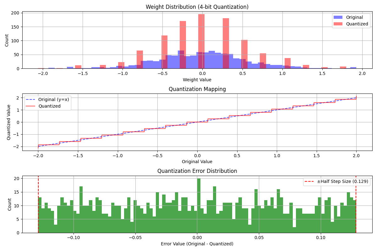
The distribution plot shows values collecting at discrete levels. The mapping plot shows the staircase produced by rounding. The error plot shows the difference between original and reconstructed values. Evenly spaced levels don’t guarantee a uniform error distribution for arbitrary inputs.
Outliers widen the range in this min-max example, increasing the distance between adjacent levels. These plots explain the numerical transformation. Model behavior requires task evaluation.
Evaluate a deployment candidate
I start with a baseline model and a public or synthetic evaluation set representative of the intended task. If memory pressure justifies quantization, I would usually evaluate an 8-bit candidate before moving to 4-bit. That order reflects my testing preference. The first comparison is less aggressive. I evaluate a 4-bit candidate when the 8-bit version leaves insufficient headroom.
Record the model revision, quantization method, runtime version, and hardware so the comparison can be repeated.
| Question | Evidence to collect |
|---|---|
| Does it fit? | Peak device memory at the intended context length and concurrency, including runtime overhead |
| Does it meet latency needs? | Time to first token and generation latency under the same load as the baseline |
| Does throughput improve? | Completed requests or output tokens per second at an acceptable latency |
| Is quality acceptable? | Task-specific correctness and failure rates on the same evaluation set |
| Does it reduce cost? | Resources needed to meet the same traffic, latency, and quality requirements |
Weight precision and compute precision can differ. For a concrete implementation, the Transformers bitsandbytes documentation describes supported 8-bit and 4-bit loading options, compute types, and hardware requirements. Select a method supported by your actual serving environment.
Connect memory savings to operating cost
Lower weight storage can create room for a larger model or a larger serving workload. Cost savings require a change in the resources you pay for or the useful work those resources deliver. A lower bill requires fewer resources or more useful work from each resource.
I call it a cost reduction after the deployment produces the same acceptable result with fewer resources or more useful work per resource.
Before adopting a candidate, compare it with the baseline under representative load and retain a rollback path. Publish the evaluation setup and measured results with any claimed savings so readers can see the conditions under which they hold.
quantization AI Model Compression LLM MLOps
842 Words
2025-01-10 21:25 +0000 (Last updated: 2026-09-17 00:00 +0000)